Course Overview > Concepts of machine learning and computer vision
Concepts of machine learning and computer vision
In this section we will discuss some important concepts on machine learning, deep learning and computer vision.
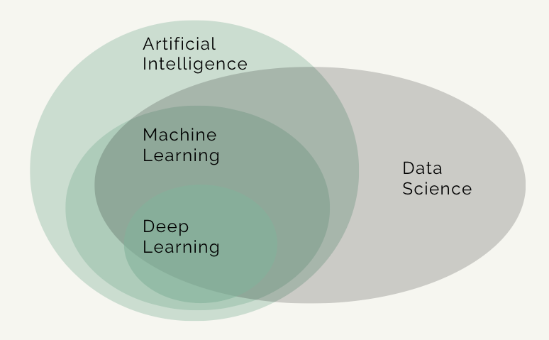
Data Science
Data science is a discipline that includes artificial intelligence (AI), machine learning (ML) and deep learning, but also some other aspects of computer science, such as algorithms, data storage and web application development. Data science is a practical discipline that requires knowledge of the domain for which it is applied for, e.g., business, medicine, biology. Data science solutions often involve AI, but usually not as much as most people would expect from the headlines.
Machine learning
Machine learning is a field of AI, while deep learning is a field of ML, although these categories are somewhat imprecise, and, for example, some parts of ML could belong to data science and statistics. Machine learning can be defined as a system that improves its performance in a given task with more experience or more data.
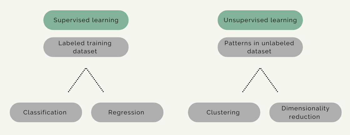
The area of ML is often divided in subareas according to the kinds of problems being solved. It can be roughly divided into supervised and unsupervised learning.
In supervised learning the model is given an input of data with known labels, for example photographs of three species of fish (label 1: species 1, label 2: species 2, label 3: species 3). The model’s task is to predict the correct label for the photograph.
In unsupervised learning there are no labels or correct outputs. The model’s task is to discover the structure of the data: for example, grouping similar items to form “clusters” or reducing the data to a smaller number of important “dimensions”. Exploratory data visualisation can be considered unsupervised learning.
The categories of supervised or unsupervised learning are not clear cut, however, and a particular method may belong to both categories. There is also a category of a so-called semisupervised learning which is partly supervised and partly unsupervised.
Each of these ML categories have different types of algorithms, which include classification, regression, clustering and dimensionality reduction. In this course we will focus primarily on supervised learning, and, in particular, classification tasks for visual data.
Computer vision is the field of research which aims to build artificial systems that can process, perceive and reason about visual data, such as images or videos. Computer vision applicaitons are rapidly increasing in our society, due to existing technological abilities to collect huge amounts of visual data. Millions of images and visual data that are generated everyday requires extensive computing resources and advanced models, if we want to make sense of it. This is what we will aim to learn in this course.
Deep learning
A technique that is widely used in computer vision these days is deep learning.
Deep learning can be defined as a system that can process and reason about data using hierarchical learning algorithms with many “layers”. This idea is loosely inspired by the way we believe our brain works. That is the reason why these algorithms are called neural networks, and are often represented by images such as the one below, showing the architecture of the algorithm.
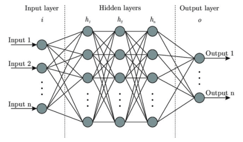 Artificial deep neural network architecture
Deep learning was first introduced and applied to a computer vision classification task in 2012 (this publication), when it just crushed the ImageNet competition, an annual Visual Classification Challenge. Researchers in this study have built and applied a deep learning algorithm called AlexNet to the ImageNet dataset. The algorithm had significantly lower error rates than other algorithms that had been applied to this dataset before.
A deep neural network is a single end-to-end pipeline that, on the left hand side (input layer), takes in the raw pixels of the image and on the right side (output layer) predicts the classification scores or probabilities. During the process of the training all parts of the algorithm are tuned and ‘trained’ simultaneously.
The input data or input layer is a column vector containing all the pixels of our input dataset. In the middle we have the hidden vectors, h, and on the right our final score vectors with classification scores per category. Generally the algorithm tries to find consistent correlations among pixels in the image, i.e. those that appear in multiple images of a specific class, but are different from images in another class.
In addition, there are weight matrices in between each of the multiple layers of the neural network. These weight matrices inform how much each element of the previous layer influences each element of the next layer.
Because of the dense connectivity pattern, this type of a neural network is typically called a fully connected network, because the units in each layer of the network are all connected to one another. Sometimes this structure is also called a “Multi Layer Perceptron or MLP”.
Convolutional Neural Networks
A convolutional neural network (also known as CNN or ConvNet) is a class of neural networks commonly applied to analyse visual imagery data.
A ConvNet is able to reduce the images into a form which is easier to process, without losing features (or variables) which are critical for getting a good prediction. Therefore, compared to other classification algorithms the pre-processing time required in a ConvNet is much lower. This is an important quality of an algorithm when we are working with massive datasets. In other words, the role of ConvNet is to decrease the computational power required to process the data through a pre-processing step of dimensionality reduction.
The convolution process uses a kernel to extract certain features from an input image. A kernel is a matrix of weights which are multiplied by the input image to extract relevant features so that the output is enhanced in a certain desirable way.
Here is a simple example of the process of convoluting a 5x5x1 image with a 3x3x1 kernel into a 3x3x1 feature.
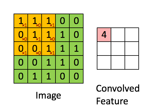
For example, the value of the first pixel (4) is derived by multiplying all the values of the kernel with the corresponding values in the pixel of the original image (1x1 + 0x1 + 1x1 + 0x0 + 1x1 + 1x0 + 0x1 + 0x0 + 1x1).
![]()
Have a look at this great online tool to visualize image kernels - you can select different kernel matrices and see how they effect the original image or build your own kernel.
You can find more information about ConvNets here.
Resources
LeCun Y, Bengio Y, Hinton G. (2015) Deep learning. Nature 521, 436–444
Rumelhart D, Hinton G, Williams R Learning (1986) Representations by Back-propagating Errors. Nature 323 (6088): 533–536
Valueva MV, Nagornov NN, Lyakhov PA, Valuev GV, Chervyakov NI (2020) Application of the residue number system to reduce hardware costs of the convolutional neural network implementation. Mathematics and Computers in Simulation, 177:232-243.